Previous Module - Next Module

Photovoltaic panels: Maximum Power Point Tracking Methods

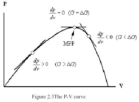
Summary

The aim of this chapter is to introduce the concept of Maximum Power Point Tracking (MPPT) of photovoltaic energy sources. The problem is described and the main techniques presented in literature are briefly explained. They are compared in order to put in evidence advantages and drawbacks of each one of them.

Drawing the maximum power from a photovoltaic panel

A photovoltaic (PV) array under uniform irradiance exhibits a current-voltage characteristic with a unique point, called the maximum power point (MPP), where the array produces maximum output power (Liu, 2002).

In Fig.1, an example of PV module characteristics and current vs. voltage for three irradiance levels S are shown. The MPP point has been also evidenced in both figures.

 

a)                                                                    b)

Figure 1. PV module characteristics for three irradiance levels S and two different panels’ temperature: a) output power vs. voltage and b) current vs. voltage.

As evidenced in Fig.1, the I-V characteristic of a PV array, and hence its MPP, changes as a consequence of the variation of the irradiance level and of the panels’ temperature, which is in turn function of the irradiance level, of the ambient temperature, of the efficiency of the heat exchange mechanism and of the operating point of the panels (Liu, 2002).

Such an effect is well described by means of Java applets. Consequently, if a PV array roughly feeds a dc source or a battery, namely operates at a fixed voltage, the power drawn from it is often sensibly less than the maximum it should be able to give if it should operate at the voltage corresponding to the MPP. Thus, it is necessary to track continuously the MPP in order to maximize the power output from a PV system, for a given set of operating conditions. The power gain an MPP tracking system is potentially able to ensure is well introduced at this page.

A dc/dc switching converter is usually entrusted with such a task: the rough source/load matching that does not ensure that the maximum power is transferred to the load at any irradiance level and temperature is removed and a switching converter is interposed between source and load in order to continuously adjust the array voltage, by changing the converter’s duty cycle, and tracking the MPP.

The issue of maximum power point tracking (MPPT) has been addressed in different ways in the literature: examples of fuzzy logic, neural networks, pilot cells and DSP based implementations have been proposed (Hohm, 2000). Nevertheless, the Perturb and Observe (P&O) and INcremental Conductance (INC) techniques are widely used, especially for low-cost implementations.

In the sequel, these two approaches to MPPT are briefly described in order to highlight their differences, advantages and drawbacks.

The incremental conductance technique

The INC algorithm is based on the observation that, at the MPP it is , where i_PV and v_PV are the PV array current and voltage respectively. From Fig.1.b it can be noted that . Therefore, named G= i_PV/v_PV and DG= |di_PV/dv_PV| the conductance and the incremental conductance of the PV field respectively, the three possible cases illustrated in the figure can occur.

When the operating point in the V-P plane is on the right of the MPP, then , whereas, when the operating point is on the left of the MPP, then . The sign of the quantity  indicates the correct direction of perturbation leading to the MPP. By means of the INC algorithm it is therefore theoretically possible to know when the MPP has been reached and therefore when the perturbation can be stopped, whereas in the P&O implementation the operating point oscillates around the MPP. Indeed, because of noise and measurement and quantization errors, the condition  is in practice never exactly satisfied, but it is usually required that such condition is approximately satisfied within a given accuracy. As a consequence, the INC operating voltage cannot be exactly coincident with the MPP and oscillates across it.

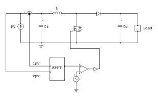
A disadvantage of the INC algorithm is in its requirements in terms of hardware and software complexity.

The Perturb and Observe (P&O) algorithm

The P&O MPPT algorithm is mostly used, due to its ease of implementation. It is based on the following criterion: if the operating voltage of the PV array is perturbed in a given direction and if the power drawn from the PV array increases, this means that the operating point has moved towards the MPP and, therefore, the operating voltage must be further perturbed in the same direction. Otherwise, if the power drawn from the PV array decreases, the operating point has moved away from the MPP and, therefore, the direction of the operating voltage perturbation must be reversed.

A drawback of P&O MPPT technique is that, at steady state, the operating point oscillates around the MPP giving rise to the waste of some amount of available energy. Several improvements of the P&O algorithm have been proposed in order to reduce the number of oscillations around the MPP in steady state, but they slow down the speed of response of the algorithm to changing atmospheric conditions and lower the algorithm efficiency during cloudy days.

Both P&O and INC methods can be confused during those time intervals characterized by changing atmospheric conditions, because, during such time intervals, the operating point can move away from the MPP instead of keeping close to it. This drawback is shown in Fig.2, where the P&O MPPT operating point path for an irradiance variation from 200W/m²to 800W/m²is reported.

a)                                                                                b)

Figure 2. P&O MPPT operating point path. The * represents MPP for different levels of the irradiance: a) slow change in atmospheric conditions, b) rapid change in atmospheric conditions

The example reports two different behaviors in the plane output power vs. voltage: Fig.2 a) shows the operating point path in presence of slowly changing atmospheric conditions, Fig.2 b), instead, shows the failure of MPPT control to follow the MPP when a rapid change in atmospheric conditions occurs. Also the INC MPPT control presents such behavior.

There is no general agreement in the literature on which of the two methods is the best one, even if it is often said that the efficiency - expressed as the ratio between the actual array output energy and the maximum energy the array could produce under the same temperature and irradiance level - of the INC algorithm is higher than that one of the P&O algorithm. To this regard, it is worth saying that the comparisons presented in the literature are carried out without a proper optimization of P&O parameters. In (Hohm, 2000) it is shown that the P&O method, when properly optimized, leads to an efficiency which is equal to that obtainable by the INC method. These are often merely chosen on the basis of trial and error tests. Unfortunately, no guidelines or general rules are provided to determine the optimal values of P&O parameters.

Paper (Femia, 2005) is devoted to fill such a hole. A theoretical analysis allowing the optimal choice of the two main parameters characterizing the P&O algorithm has been carried out. The key idea underlying the proposed optimization approach lies in the customization of the P&O MPPT parameters to the dynamic behavior of the whole system composed by the specific converter and PV array adopted. Results obtained by means of such approach clearly show that, in the design of efficient MPPT regulators, the easiness and flexibility of P&O MPPT control technique can be exploited by optimizing it according to the specific system’s dynamic.

As an example, the boost converter reported in Fig. 3(a) is examined. Results obtained and the considerations that are drawn can be extended to any other converter topology as well.

(a)                                                                                          (b)

Figure 3. Boost converter with MPPT control: a) simplified circuit, b) equivalent block diagram.

The system in Fig. 3(a) can be schematically represented as in Fig. 3(b), where d is the duty cycle and p is the power drawn from the PV array. In the following, the sampling interval will be indicated with T_a, and the amplitude of the duty cycle perturbation with Dd=|d(kT_a)-d((k-1)T_a)|>0.

In the P&O algorithm the sign of the duty cycle perturbation at the (k+1)-th sampling is decided on the basis of the sign of the difference between the power p((k+1)T_a) and the power p(kT_a) according to the rules discussed above:

d((k+1)T_a)=d(kT_a)+(d(kT_a)-d((k-1)T_a))×sign(p((k+1)T_a)-p(kT_a))                                                        (1)

The amplitude of the duty cycle perturbation is one of the two parameters requiring optimization: lowering Dd reduces the steady-state losses caused by the oscillation of the array operating point around the MPP; however, it makes the algorithm less efficient in case of rapidly changing atmospheric conditions. The optimal choice of Dd in these situations, when we have to account for both the source’s and converter’s dynamics, is discussed in detail in (Femia, 2005). Besides the case of quickly varying MPP, which occurs in cloudy days only, there is a more general problem, connected to the choice of the sampling interval T_a used by the P&O MPPT algorithm, which arises even during sunny days, when the MPP moves very slowly. The sampling interval T_a should be set higher than a proper threshold in order to avoid instability of the MPPT algorithm and to reduce the number of oscillations around the MPP in steady state. In fact, considering a fixed PV array MPP, if the algorithm samples the array voltage and current too quickly, it is subjected to possible mistakes caused by the transient behavior of the whole system (PV array+converter), thus missing, even if temporarily, the current MPP of the PV array, which is in steady-state operation. As a consequence, the energy efficiency decays as the algorithm can be confused and the operating point can become unstable, entering disordered and/or chaotic behaviors. To avoid this, it must be ensured that, after each duty-cycle perturbation, the system reaches the steady-state before the next measurement of array voltage and current is done. In (Femia, 2005) the problem of choosing T_a is analyzed and an optimized solution, based on the tuning the P&O algorithm according to converter’s dynamics, is proposed. In (Femia, 2005) the optimization procedure is illustrated for rapidly varying irradiance conditions; simulation results have been validated by experimental verifications.

References

N.Femia, G.Petrone, G.Spagnuolo, M.Vitelli (2005), Optimization of Perturb and Observe Maximum Power Point Tracking Method, IEEE Transactions on Power Electronics, Vol.20, N.4, July 2005, pp.963-973.

D.P.Hohm, M.E.Ropp (2000): “Comparative Study of Maximum Power Point Tracking Algorithms”, Conference Record of the Twenty-Eighth IEEE Photovoltaic Specialists Conference, September 2000, pp.1699-1702.

S. Liu, R. A. Dougal (2002), Dynamic multiphysics model for solar array, IEEE Trans. On Energy Conversion, Vol. 17, No. 2, June 2002, pp. 285-294.

Top - Previous Module - Next Module