(paper abridged to 5 pages)

Ion V. Ion, Spiru Paraschiv, Daniela Negoita, Ion C. Ionita - „Lower Danube” University of Galati – Romania

ion.ionita@ugal.ro

Introduction. The strong connection between cost and quality

How about HSVs? HSVs are of course, products, but they are manufactured and sold to deliver a service, namely to transport people or goods. In fact all the products are bought to make a service, the final destination of every product is to serve people someway.

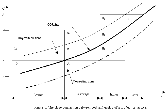
Between cost and quality of every product or service there is a strong connection, as we can see from Fig.1. Here are plotted the costs C versus the quality Q of the goods or services. The sloping line CQR (cost-to-quality ratio) expresses just the connection between the two main features of any product or service, namely cost C and quality Q. For the quality Q were drawn four usual zones: Lower, Average, Higher and Extra. Of course, this conventional division is done for analytical purposes, because the inter-boundaries are imaginary, in fact the transition from one to the next category being smoothly. The focus area of the graph is the box A2, associated to an average quality of the product or service with corresponding cost C=2…3. In box A3 are the products made at the same average quality but with higher cost C=3…4, reason for which they are not profitable. In box A1 are placed the products or services of average quality, made with low costs. That's why these products or services are very interesting and profitable, therefore competitive. On the left-hand side of the graph we can see the products or services by lower quality. Box L1 represents the qualitatively inadequate products or services, made with minimal cost C=1…2. It is true that on some markets such products or services are abundant. Box L2 includes both qualitatively and economically inadequate products or services. They are made with lower quality but with relative high costs, which means that production or service delivering like this is not profitable. On the right-hand side of the graph we can find the products or services of superior quality. The box labeled H2 includes the higher quality products or services, with costs C=3…4, that match their quality. In box H3 there are higher quality products or services indeed, but unprofitable, because they are hardly to sell, or not saleable at all. The box H1 accounts for superior and inexpensive products or services. They are easily saleable, and very competitive.At last, box E1 represents the most expensive products or services, of extra quality. These are luxury products.Let's notice the continuous increasing of the CQR line slope. That is the quality cost, establishment we knew before, and this is just a confirmation.

Reading Figure 1 in horizontal direction we note the relative values of the cost C. The products made with low costs C=1…2 are reminding us of minimum cost optimization. Here it is important to note, however, that in the box L1 there are qualitatively inadequate products, and that only the products or services of average quality (A1) are competitive. We reached here the matter of our paper: the optimization of any beneficial activity should be made not only on a cost basis, but also by considering in the same measure the quality of the products or services. In terms of HSV, the higher is the construction complexity of the car the more expensive it is. But this general tendency is much influenced by the market competition.

In the graph of Figure 1 we can notice the upper left-hand zone, situated above CQR line, that is the unprofitable zone of goods or services. Meanwhile, the lower right-hand side zone, situated below CQR line, represents competitive products and services, of superior quality and made with lower costs. To know that an HSV is profitable, the buyer has to see that his purchase is situated as right-hand side as possible (better quality) and as low as possible (cheaper). More about this topic can be found in reference [4].

2.Structuring the cost-to-quality ratio

Being conscious that every payment act is done in fact in terms of cost-to-quality ratio, when analyzing a HSV we have carefully formulate the cost-to-quality ratio of the analyzed car. We have to do this having permanently in view how the customer will pay that HSV. For instance, there is no sense to calculate the production of a HSV factory in terms of [€/hour] and not having in view the real cost of what it produces, that is the individual cost expressed in [€/HSV].

In the case of the transport service, the final cost must be expressed in [€/km]. Here “km” means a 1 km distance, covered by a certain HSV, characterized by the very well specified quality parameters.

We have to end this section by noticing that always a payment act, as result of sailing, is done in terms of cost-to-quality ratio [€/car or €/km], never in terms of cost [€], not related with the quality of what was paid.

3.The quality parameters of a HSV

As product a HSV must accomplish the following quality parameters: QP01–Accessibility; QP02–Adaptability; QP03–Availability; QP04–Cleanliness; QP05–Credibility; QP06–Durability; QP07–Environmental Protection; QP08–Fuel Consumption; QP09–Functional Engine Parameters; QP10–Inflammability; QP11–Lighting Parameters; QP12–Look; QP13–Maintainability; QP14–Parking Capacity; QP15–Productivity; QP16–Promptitude; QP17–Protection; QP18-PV Panel Parameters; QP19-Reliability; QP20–Safety; QP21–Size; QP22–Style; QP23–Susceptibility; QP24–Pneumatic Tires Parameters; QP25–Toxicity; QP26–Transportability; QP27–Transport Capacity; QP28–Vulnerability; QP29–Watching capacity; QP30–Weight; QP31–Workings.

As the service that HSVs must deliver (namely transport), they have the following quality parameters: QS01–Accessibility; QS02–Accuracy; QS03–Comfort; QS04–Competence; QS05–Confidence; QS06–Credibility; QS07–Efficacy; QS08–Efficiency; QS09–Feedback speed; QS10–Formalism; QS11–Honesty; QS12–Proficiency; QS13–Promptitude; QS14–Punctuality; QS15–Safety.

In the above listed quality parameters, the cost C of the product or of the service is not at all mentioned. Why? Because the cost is expressing all the efforts done to accomplish the quality requirements, it has a component in each of the above-mentioned items.

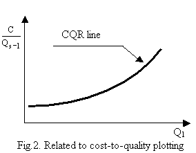
Now, let us propose to represent graphically the dependence cost versus quality, according to fig.1, that is, using a two dimensional (2D) space. If we denote by s-the number of the above mentioned quality parameters and reserve for the cost C one dimension, that means we have to operate in the space of (s+1) dimensions, but we know that we are not able to operate in a space with more than 3 dimensions (3D). To draw in cost-to-quality coordinates that is in (2D) space, we have to evaluate quality by only one value. This is possible only if all the quality features will have the same measure unit, requirement which is very difficult to reach. There is still a possibility, namely when will give to each quality feature a number of points and finally will express the quality summing all the features points. This procedure is so far arbitrary, we will use it only if we shall not have another else better. To exceed this difficulty we shall to remember that in fact the cost C is not a single parameter having the measure unit [€], but it is in fact a parameter of cost-to-quality ratio, in terms of [$/kWh], [$/kg] and so on. That means that in ordinate axis of C we shall put not a simple amount of money [$], but a cost-to-quality ratio C/Q that is a unitary cost of the car (€/car) or of the transport (€/km).To this purpose all the s quality features of a product or service are divided into two distinct categories:

-the group of s-1 implicit demands that represent the product (car) or the service (transport);

-one single quality demand Q₁ that differentiates cars or transports among them ( for instance the inner individual space [cube meter/person]).

This separation of the quality features is done in order to make comparable the single feature Q₁ of the product or service (Fig.2).To be comparable, all the compared products or services must have the rest of  (s-1) features of the same or about same correspondent values.

4. The cost structure

c_p,s = C_F + c_I +c_OM         [€/car or €/km]                                                                         (5)

The term c_F includes all the energy (fuel, electricity) and all the matter consumed to complete the product or to deliver the service. The term c_I [€/car or €/km] includes all the investment expenditures done to complete the product or to deliver the ordered service. The term c_OM [€/car or €/km] includes all the expenditures done to complete the product or the service and which are not included in the previously formulated two terms: c_F and c_I. In the operation-maintenance cost component are included: all the employed people salaries, all the equipment and buildings maintenance costs, taxes, fines, even the preferred foot-ball team financial support. The components C_F, C_I and C_OM  must be calculated as cost-to-quality ratios as they are, that is, in terms of [€/car or €/km].

5. The matter of the compared cost-to-quality analysis of the HSV_s

This analysis procedure starts from the end-user demands, because he is the HSV payer. It is very well known, that the aim of every production is to make profit. But to do this, we have to satisfy these payer's demands, which are the quality parameters of the HSV for sale or of the transport service to be delivered. Never a payer will give a cent without knowing very well the quality parameters of the bought HSV. When we buy a HSV, we pay Euros per HSV [€/car]. Let us think that every paid car means in fact a bunch of quality parameters defining that car.

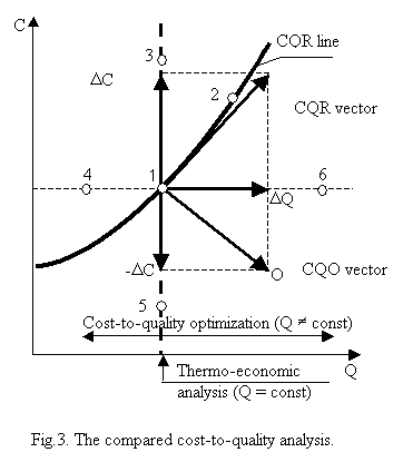
To present more clearly the compared cost-to-quality analysis procedure let's presume that we studied 6 different variants of HSV and we have calculated the corresponding cost-to-quality ratios (the points 1-6 in Fig.3). We can see that thermo-economics [1,7,8,9] operates along the vertical line of variable cost C and constant quality Q, while the compared cost-to-quality analysis operates on the surface defined by variable cost C and variable quality Q. Now to go ahead we need to remember the strong connection between cost and quality of any product or service.

Coming back to Fig.3, we can draw the lowering cost vector  and write the vector equation

                                        (4)

The resultant vector  is cost-to-quality optimization vector, which is aiming to low the cost C and to increase the quality Q. That means that if we have 6 different points 1; 2; 3; 4; 5 and 6 in the C vs. Q diagram, the points 4 and 3 are located in the unprofitable zone, while the points 5 and 6 are placed in the competing zone. Which of the points 5 or 6 will be chosen by the end user? It is a problem of his material possibilities and of the wished quality. More about this the reader can find in [11].

Nomenclature

Latin letters: C – total cost, [€/car]; c_F – the energy or matter cost, [€/car or €/km]; c_I – the investment cost, [€/car or €/km]; c_OM – the operation-maintenance cost, [€/car or €/km]; c_P,C_S – the total cost of a product (car) and service (km of transport) respectively, [€/car or €/km]; CQO-cost-to-quality optimization; CQR-cost-to-quality ratio; HSV-hybrid solar vehicle; QP –product (car) quality parameter; QS- service (transport) quality parameter;

Greek letters: ΔC-cost variation; ΔQ-quality variation.

Subscripts: F –energy (fuel or electricity), consumption materials; I – investment; OM – operation-maintenance;

P – product; S – service;

References

1. Sciubba E. and Melli R. (1998), Artificial Intelligence in Thermal Systems Design: Concepts and Applications, Nova Science Publishers, Inc., New York

2. Ionita C.I., Ion V.I. (1999), Cost/Quality Ratio (CQR), a Comprehensive Value of the Thermal Production Optimization, 4^th Conference on Heat Engines and Environmental Protection, May 31– June 2, 1999, Hotel Uni, Balatonfüred, Hungary, Proceedings, pp.187-188.

3. Ionita C.I. (2001), The Close Connection between Cost and Quality of Energy Products, ECOS 2001, Istanbul, Proceedings, vol.2, pp.813-820.

4. Ionita C.I., Popa.V.(2000), The Analysis of the hvac Systems Using Cost-to-Quality Criterion of Optimization, 7^th REHVA World Congress Clima 2000, Napoli 2001, Proceedings on CD.

5. Ionita C.I. (2003), Engineering and Economic Optimization of Energy Production, International Journal of Energy Research, Article Reference No.811, Journals Production Dept., 26: 697-715 (DOI: 10.1002/er.811), John Wiley&Sons, Ltd, Chichester, UK.

6. Ionita C.I. (2001), The Cost-to-Quality Ratio Based Optimization of the Energy Production, Entropie nr.232, 2001, pp.10-19.

7. Bejan A., e.a. (1996) – Thermal Design & Optimization, John Willey & Sons, New York

8. Sciubba E. (2001), From Engineering Economics to Extended Exergy Accounting: the Path from “Monetary Cost” to “Resource-Based Value, Ecos'01, July 4-6 2001, Istanbul, Proceedings, vol.1, pp.21-37.

9. Valero A., Botero E. (2002), An Assessment of the earth's clean fossil exergy capital based on exergy abatement costs, ECOS 2002, Berlin, Germany, Berlin, Germany, Proceedings, pp.151-157.

10. Ioniţă,C.I.(2002)“Extending thermo-economic analysis by cost to quality optimisation”. Proceedings of ECOS 2002 July 3-5, 2002, Berlin, Germany, pag.1434-1441.

11. Ionita C.I.,Ion V.I.,Iosifescu Cr.,Popa V. “Cost-to-Quality Optimization of Refrigeration” in Low Temperature and Cryogenic Refrigeration”NATO Science Series II-vol.99 Kluwer Academic Publishers, Dordrecht/Boston/London (2002), ISBN 1-4020-1273-X(HB); ISBN 1-4020-1274-8(PB).

12. Ionita C.I.(2003) “Exergetical Cost-to-Quality-Analysis of an Autonomous Apartment Heating” ECOS 2003, Copenhagen, Denmark, 2003, Proceedings, pag-649-656.

13. Ionita C.I., (2003), “From Energy Analysis to Compared Cost-to-Quality Analysis of the ThermalSystems”, Technical Sciences Academy of Romania, MOCM-9-vol.2, pp.149-155, ISSN 1224-7480.

14. Ionita C.I., (2004) “The Compared Cost-to-Quality Analysis in Mechanical Engineering” Buletinul Institutului Politehnic Iasi,Tomul L(LIV),Fasc.6C,2004,Sectia Constructii de Masini,p.13-20.

15. Ion Ioniţă (2005) “Beyond thermo-economic analysis of thermal systems: the compared cost-toquality analysis”, 1^st International Conference on Thermal Engines and Environmental Engineering, June 3-4, 2005, Galati, Romania (Proceedings on CD).

P.S. There is, also, the unabridged work with the same title “The Compared Cost-to-Quality Analysis of HSVs”. Its length is 10 pages and the name of document is “The compared cost - unabridged.”

Inizio Pagina - Modulo Precedente